Optimal Control Problem and LQR
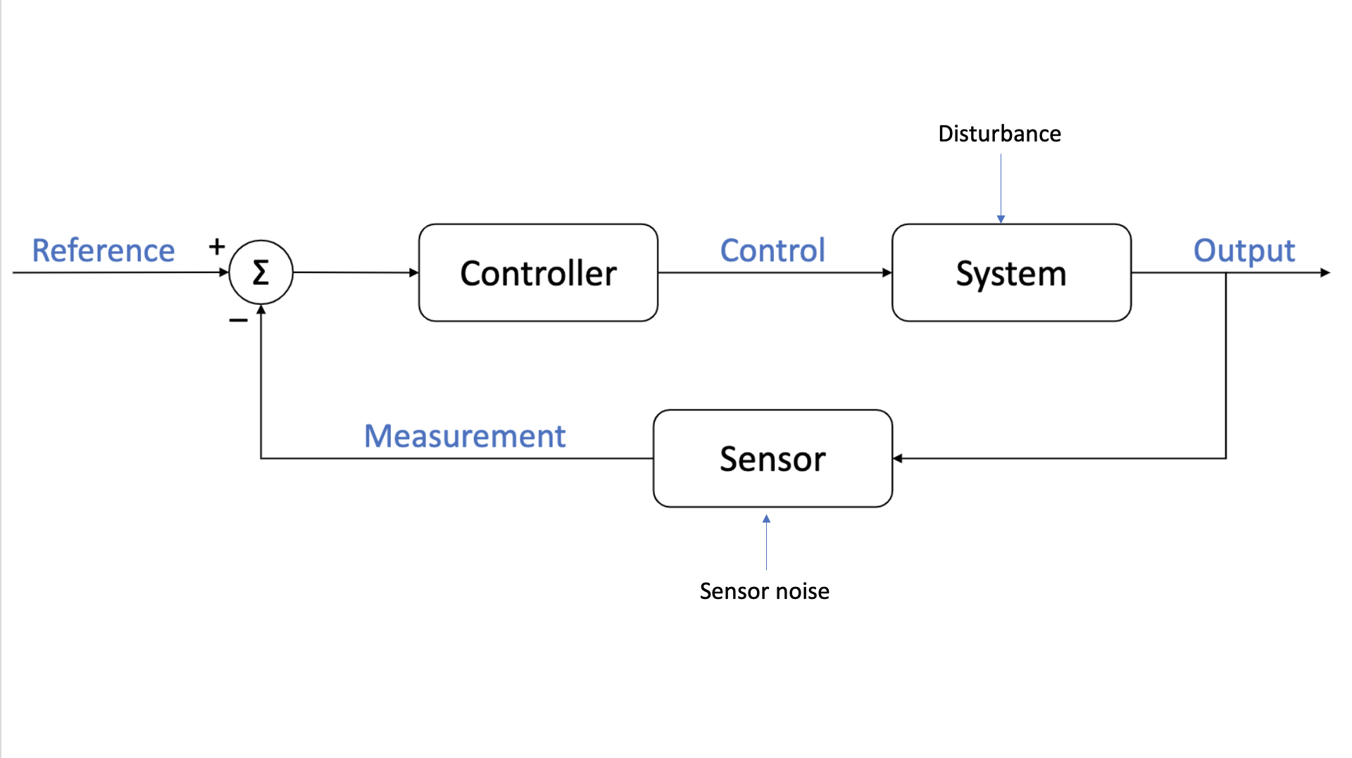
Feedback Control


State-Space Models
\[\boldsymbol{\dot{x}}(t)=f(\boldsymbol{x}(t), \boldsymbol{u}(t),t)\]- a history of control input values during the interval $[t_0,t_f]$ is called a control histroy and is denoted by \(\boldsymbol{u}\)
- a history of state values during the interval $[t_0,t_f]$ is called a state trajectory and is denoted by $$\boldsymbol{x}$$
Speed, Accelerator as Example
Recall:
\[\ddot{s}(t)=a(t)\]\(\begin{bmatrix}\dot{s}\\ \dot{v} \end{bmatrix}=\begin{bmatrix}v\\ a \end{bmatrix}\) \(\begin{bmatrix}\dot{s}\\ \dot{v} \end{bmatrix}=\begin{bmatrix}0&1\\ 0&0\end{bmatrix}\begin{bmatrix}s\\ v\end{bmatrix}+\begin{bmatrix}0\\ 1\end{bmatrix}a \\ \boldsymbol{\dot{x}}(t)=A\boldsymbol{x}(t)+B \boldsymbol{u}(t) \\ \begin{bmatrix}\dot{\boldsymbol{s}}\\ \dot{\boldsymbol{v}} \end{bmatrix}=\begin{bmatrix}0&I\\ 0&0\end{bmatrix}\begin{bmatrix}\boldsymbol{s}\\ \boldsymbol{v}\end{bmatrix}+\begin{bmatrix}0\\ 1\end{bmatrix}\boldsymbol{a} \\\) Drive from \([5,0]^T\) to \([0,0]^T\).
Use a linear feedback control law. \(a=-k_ps-k_dv\\ \begin{bmatrix}\dot{s}\\ \dot{v} \end{bmatrix}=\begin{bmatrix}0&1\\ 0&0\end{bmatrix}\begin{bmatrix}s\\ v\end{bmatrix}-\begin{bmatrix}0\\ 1\end{bmatrix}\begin{bmatrix}k_p&k_d\end{bmatrix}\begin{bmatrix}s\\v\end{bmatrix} \\ \begin{bmatrix}\dot{s}\\ \dot{v} \end{bmatrix}=\begin{bmatrix}0&1\\ -k_p&-k_d\end{bmatrix}\begin{bmatrix}s\\ v\end{bmatrix}\\ \dot{\boldsymbol{x}}(t)=(A-BK)\boldsymbol{x}(t)\)
Optimal Control Problem
Continuous Time
Continuous-time systems dynamics as \(\boldsymbol{\dot{x}}(t)=f(\boldsymbol{x}(t), \boldsymbol{u}(t),t)\)
Performance measure: \(J=c_f(\boldsymbol{x}(t_f),t_f)+\int_{t_0}^{t_f}c(\boldsymbol{x}(t),\boldsymbol{u}(t),t)dt\) c - instantaneous cost function
\(c_f\) - terminal state cost
Find an admissible control, \(\boldsymbol{u}^*\), which caused the system to follow an admissiable trajectory, \(\boldsymbol{x}^*\), that minimizes the performance measure. The minimiser (\(\boldsymbol{x}^*,\boldsymbol{u}^*\)) is called an optimal trajectory-control pair.
Discrete Time
Discrete-time systems dynamics as \(\boldsymbol{x}_{k+1}=f_k(\boldsymbol{x}_k, \boldsymbol{u}_t)\)
Performance measure: \(J=c_N(\boldsymbol{x}_N)+\sum_{k=0}^{N-1}c(\boldsymbol{x}_k,\boldsymbol{u}_k,k)\) c - stage-wise cost function
\(c_N\) - terminal cost function
Optimal Control(Open Loop)
\[\min_{x,u}\sum_{t=0}^{T}c_t(x_t,u_t)\\ s.t. \ x_0=\overline{x_0}\\ x_{t+1}=f(x_t,u_t) \ t =0,...,T-1\]Non-convex optimization problem, can be solved with sequential convex programming(SCP)
Optimal Control(Close Loop)
Given: \(\overline{x_0}\)
For $&t=0,1,2,…,T$$
Solve \(\min_{x,u}\sum_{t=0}^{T}c_t(x_t,u_t)\\ s.t. \ x_{k+1}=f(x_k,u_k), \forall k \in \{t,t+1,...,T-1\}\\ x_t=\overline{x_t}\) Execute \(u_t\)
Observe resulting state, \(\overline{x_{t+1}}\)
Initialize with solution from \(t-1\) to solve fast at time \(t\)
Markovian Decision Problems
The fundamental idea behind Markov Decision Processes (MDPs) is that the state dynamics are Markovian, or obey the Markov property. This property says that all information about the previous history of the system is summarized by its current state. \(\boldsymbol{x}_{k+1}=\boldsymbol{f}_k(\boldsymbol{x}_k,\boldsymbol{u}_k,\boldsymbol{w}_k)\) $\boldsymbol{w}_k$ - stochastic disturbance, with \(\boldsymbol{w}_j\) independent of \(\boldsymbol{w}_i\) for \(i\neq j\). \(\boldsymbol{h}_k=(\boldsymbol{x}_0,\boldsymbol{u}_0,c_0,...,,\boldsymbol{u}_k)\) \(c_i\) - accrued cost at timestep i
A system is said to be Markovian if \(p(\boldsymbol{x}_{k+1}|\boldsymbol{x}_{k},\boldsymbol{u}_{k})=p(\boldsymbol{x}_{k+1}|\boldsymbol{h}_{k})\) In addition to Markovian dynamics, we require an additive cost function, \(c(\boldsymbol{x}_k,\boldsymbol{u}_k, k)\).
Define the Markov process as the tuple \((\mathcal{X},\mathcal{U},\boldsymbol{f},c)\).
\(\mathcal{X}\) - State space, \(\boldsymbol{x}_t \in \mathcal{X}\)
\(\mathcal{U}\)- action space, \(\boldsymbol{u}_t \in \mathcal{U}\)
Something missing:
- constraints
- final time
- initial state
Linear case: LQR
Linear - linear system dynamics
Quadratic - quadratic cost
Regulator - regulating signal of a system
Very speical case: Optimal Control for Linear Dynamic Systems and Quadratic Cost(a.k.a. LQ setting)
Four sub-types:
Discrete-time Deterministic LQR
Discrete-time Stochastic LQR
Continuous-time Deterministic LQR
Continuous-time Stochastic LQR
Deterministic - Nosieless
Stochastic - Noise
Discrete-time Time-Varying Finite-Horizon Linear System